Search DynamoDB Data with Amazon Elasticsearch Service
Introduction
Overview
This lab imagines a scenario where you are running an online store that sells movies for streaming. Using a common pattern, you will store your movie catalog in an Amazon DynamoDB table (DynamoDB). In order to provide relevant, text-based querying, you will replicate the data in an Amazon Elasticsearch Service (Amazon ES) domain.
Topics covered
By the end of this lab you will be able to:
- Create a DynamoDB table
- Connect your table to an Amazon ES domain
- Write complex queries and adjust relevance
- Stream changes from your DynamoDB table to your Amazon ES domain and monitor clicks and purchases
Prerequisites
Some familiarity with AWS CloudFormation is recommended
Amazon Elasticsearch Service
Amazon Elasticsearch Service introduction
Amazon Elasticsearch Service is a managed service that makes it easy to deploy, operate, and scale Elasticsearch in the AWS cloud. Elasticsearch is a popular open-source search and analytics engine for use cases, such as log analytics, real-time application monitoring, click stream analytics, and text search.
With Amazon Elasticsearch Service, you get direct access to the Elasticsearch open-source APIs so that existing code and applications will work seamlessly. You can set up and configure your Amazon Elasticsearch cluster in minutes from the AWS Management Console.
Amazon Elasticsearch Service provisions all the resources for your cluster and launches it. Amazon Elasticsearch Service automatically detects and replaces failed Amazon Elasticsearch nodes, reducing the overhead associated with self-managed infrastructures. You can deploy an Amazon Elasticsearch cluster in minutes using the AWS Management Console. There are no upfront costs to set up Amazon Elasticsearch clusters, and you pay only for the service resources that you use.
The service offers integrations with open-source tools like Kibana and Logstash for data ingestion and visualization. It also integrates seamlessly with other AWS services such as Amazon Virtual Private Cloud (VPC), AWS Key Management Service (KMS), Amazon Kinesis Data Firehose, AWS Lambda, AWS Identity and Access Management Service (IAM), Amazon Cognito, and Amazon CloudWatch, so you can go from data to actionable insights quickly and securely.
Amazon Elasticsearch Service offers the following benefits of a managed service:
- Simple cluster scaling via API
- Self-healing clusters
- High availability on-demand
- Automatic cluster snapshots for data durability
- Security
- Cluster monitoring
Components of Amazon Elasticsearch Service
Amazon Elasticsearch Service contains the following components:
Domain: An Amazon Elasticsearch domain comprises an Elasticsearch cluster – hardware and software – along with additional hardware and software providing load-balancing, security, and monitoring. The domain is exposed by service endpoints for Amazon Elasticsearch Service.
Cluster: A cluster is a collection of one or more data nodes, optional dedicated master nodes, and storage required to run Elasticsearch.
Node: A node is single instance within an Elasticsearch cluster that has the ability to recognize and process or forward messages to other nodes.
Storage: Amazon Elasticsearch Service supports two distinct storage types, the Instance (default) storage or Elastic Block Store (EBS) – general purpose (SSD), provisioned IOPS (SSD), and magnetic.
Amazon DynamoDB
Amazon DynamoDB introduction
Amazon DynamoDB is a fully managed NoSQL database service that provides fast and predictable performance with seamless scalability. DynamoDB lets you offload the administrative burdens of operating and scaling a distributed database, so that you don’t have to worry about hardware provisioning, setup and configuration, replication, software patching, or cluster scaling. Also, DynamoDB offers encryption at rest, which eliminates the operational burden and complexity involved in protecting sensitive data.
With DynamoDB, you can create database tables that can store and retrieve any amount of data, and serve any level of request traffic. You can scale up or scale down your tables’ throughput capacity without downtime or performance degradation, and use the AWS Management Console to monitor resource utilization and performance metrics.
Amazon DynamoDB provides on-demand backup capability. It allows you to create full backups of your tables for long-term retention and archival for regulatory compliance needs. You can create on-demand backups as well as enable point-in-time recovery for your Amazon DynamoDB tables. Point-in-time recovery helps protect your Amazon DynamoDB tables from accidental write or delete operations. With point-in-time recovery, you can restore that table to any point in time during the last 35 days.
DynamoDB allows you to delete expired items from tables automatically to help you reduce storage usage and the cost of storing data that is no longer relevant.
Components of Amazon DynamoDB
The following are the basic DynamoDB components:
Tables – Similar to other database systems, DynamoDB stores data in tables. A _table_ is a collection of data. For example, you can create a table called Movies that you could use to store a collection of movies to support your eCommerce application. You could also have a _Theaters_ table to store information about where the movies are playing.
Items – Each table contains zero or more items. An _item_ is a group of attributes that is uniquely identifiable among all of the other items. In a _Movies_ table, each item represents a movie. For a Theaters table, each item represents one theater. Items in DynamoDB are similar in many ways to rows, records, or tuples in other database systems. In DynamoDB, there is no limit to the number of items you can store in a table.
Attributes – Each item is composed of one or more attributes. An _attribute_ is a fundamental data element, something that does not need to be broken down any further. For example, an item in a Movies table contains attributes called Title, description, rating, price, and so on. For a _Theaters_ table, an item might have attributes such as Address, _Number_ofScreens, Manager, and so on. Attributes in DynamoDB are similar in many ways to fields or columns in other database systems.
When you create a table, in addition to the table name, you must specify the primary key of the table. The primary key uniquely identifies each item in the table, so that no two items can have the same key.
DynamoDB supports two different kinds of primary keys:
Partition key – A simple primary key, composed of one attribute known as the partition key.
DynamoDB uses the partition key’s value as input to an internal hash function. The output from the hash function determines the partition (physical storage internal to DynamoDB) in which the item will be stored.
In a table that has only a partition key, no two items can have the same partition key value.
The People table described in Tables, Items, and Attributes is an example of a table with a simple primary key (PersonID). You can access any item in the People table directly by providing the PersonId value for that item.
Partition key and sort key – Referred to as a composite primary key, this type of key is composed of two attributes. The first attribute is the partition key, and the second attribute is the sort key.
DynamoDB uses the partition key value as input to an internal hash function. The output from the hash function determines the partition (physical storage internal to DynamoDB) in which the item will be stored. All items with the same partition key are stored together, in sorted order by sort key value.
In a table that has a partition key and a sort key, it’s possible for two items to have the same partition key value. However, those two items must have different sort key values.
The Music table described in Tables, Items, and Attributes is an example of a table with a composite primary key (Artist and SongTitle). You can access any item in the Music table directly, if you provide the Artist and SongTitle values for that item.
A composite primary key gives you additional flexibility when querying data. For example, if you provide only the value for Artist, DynamoDB retrieves all of the songs by that artist. To retrieve only a subset of songs by a particular artist, you can provide a value for Artist along with a range of values for SongTitle.
Both Amazon DynamoDB and Amazon ES are databases. You use their APIs to send and store data, as well as query that data. However, they provide different and complementary capabilities, especially when it comes to searching the underlying data. When you have textual data or many structured fields, you use DynamoDB as a primary, durable store and Amazon ES to provide search for your data.
Lab overview
[](../assets/image001.png)
In the lab you will deploy a CloudFormation stack that will create resources for you in AWS. It deploys a Lambda function (Lambda Stream Function), triggered by DynamoDB table’s stream. It deploys a second Lambda function (Lambda Wiring Function) that reads the source data from S3 (#1) and loads it into the DynamoDB table (#2). The Lambda stream function, which is already in place, catches the updates to the table and inserts the records into Amazon ES (#3). Finally, you will run a third Lambda function (Lambda Streaming Function) to generate updates to the DynamoDB table (#4), which the Lambda stream function will propagate to Amazon ES.
The source data is a set of 246, Sci-Fi/Action movies, sourced from IMDb. The Lambda wiring function reads this data, adds clicks, price, purchases, and a location field, and creates the item in the DynamoDB table.
The DynamoDB schema uses the movie’s id as the primary key and adds items for the movie data’s fields.
{
“id”: “tt0088763”,
“title”: “Back to the Future”,
“year”: 1985,
“rating”: 8.5,
“rank”: 204,
“genres”: [
“Adventure”,
“Comedy”,
“Sci-Fi”
],
“plot”: “A teenager is accidentally sent 30 years into the past in a time-traveling DeLorean invented by his friend, Dr. Emmett Brown, and must make sure his high-school-age parents unite in order to save his own existence.”,
“release_date”: “1985-07-03T00:00:00Z”,
“running_time_secs”: 6960,
“actors”: [
“Christopher Lloyd”,
“Lea Thompson”,
“Michael J. Fox”
],
“directors”: [
“Robert Zemeckis”
],
“image_url”: “http://ia.media-imdb.com/images/M/MV5BMTk4OTQ1OTMwN15BMl5BanBnXkFtZTcwOTIwMzM3MQ@@._V1SX400.jpg”,
“location”: “44.54, -67.0 “,
“purchases”: 12460,
“price”: 29.99,
“clicks”: 1277594
}
These fields will also serve as the basis for querying the data in Elasticsearch.
Step 1: Launch the CloudFormation stack
Using a web browser, login to the AWS Console at https://console.aws.amazon.com/
Choose EU (Ireland) in the region selector
Go to the CloudFormation console
Choose Create Stack
In the resulting window, select Specify an Amazon S3 template URL. Use the following template: https://s3.amazonaws.com/imdb-ddb-aes-lab-eu-west-1/Lab-Template.json
Enter a Stack Name.
You can leave the other template parameters at their defaults or choose your own.
Click Next
Leave all the defaults on this page. Scroll to the bottom of the page and click Next
On the next page, click the checkbox next to I acknowledge that AWS CloudFormation might create IAM resources with custom names
Click Create
The stack will take approximately 15 minutes to deploy.
Examine the CloudFormation template
While the lab stack deploys, let’s examine the template along with the Lambda functions it creates. The stack contains a set of Mappings, Parameters, and Resources. The Mappings tell CloudFormation which S3 bucket contains the Lambda code, based on the region you select in the console. The Parameters are straightforward, letting you give your stack a prefix and control the index name for the movies index in your Amazon Elasticsearch Service domain.
CloudFormation Resources are the AWS resources deployed. You specify these resources with a set of parameters that you supply in the source JSON or yml. CloudFormation works out the resource dependencies and makes sure that resources deploy in the correct order. There are 12 resources in this template.
CognitoUserPool – The lab deploys Cognito resources to supply the basis for authenticating to Kibana. The user pool controls user sign on.
CognitoIdentityPool – The identity pool is the source of Cognito identities.
ElasticsearchDomain – Your Elasticsearch domain. NOTE: The AuthUserRole and the domain’s policy are the key components that enable Cognito access. The Principal for this role is Cognito’s default, AuthUserRole. All users who authenticate through Cognito get this role (unless you specify otherwise). These two pieces are what you need to enable Cognito access in Kibana for your own domains. You can read more in our documentation.
DDBTable – The Dynamo DB table. There are a couple of parameters to note here: the template specifies the primary key (a hash called “id”). More important, it has a StreamSpecification that directs all NEW_AND_OLD_IMAGES to the attached stream. This setting means that updates will come to the LambdaStreamFunction with both the existing and new image. The Lambda function uses both of these to send deltas to Amazon ES.
FunctionSourceMapping – attaches the LambdaFunctionForStreaming to the Dynamo DB table. This completes the setup of the infrastructure to transfer changes to the Dynamo table, as posted to the DDB Stream, to the Amazon ES domain.
AuthUserRole – This role is assigned to authenticated Cognito users and allows them to access Cognito resources.
IdentityPoolRoleAttachment – This attaches the role to the identity pool.
LambdaExecutionRole – all Lambda functions in the lab use this role, making it wider than you should use in your own Roles.
Lambda code
CloudFormation creates three Lambda functions to perform various tasks. You can view these Lambda functions in your Lambda console and see the code.
The most interesting of these functions is the LambdaWiringFunction. This function is called when CloudFormation creates the stack. It sends a mapping to the Amazon ES, setting types for the movie data’s fields. It downloads and sends the movie data to Dynamo DB. Finally, it performs two functions not supported in CloudFormation – creating a Cognito domain for supporting the login UI and creating a Cognito user.
It’s very useful to create small functions like these to augment CloudFormation’s template creation, whether inline or in S3. Pay particular attention to the handler function, and the send_response function. It is critically important that all code paths eventually return a value to CloudFormation, or the template will not create or delete correctly.
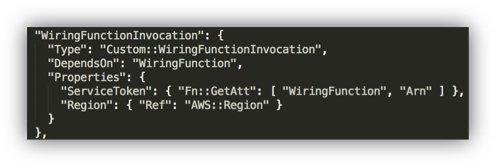
In the template, pay attention to the WiringFunctionInvocation. You need this to get CloudFormation to call your custom Lambda resource.
Another useful pattern is to pass the various CloudFormation resource names and ARNs to the Lambda function via environment variables. Note that the wiring function passes many values this way.
The LambdaFunctionForDDBStreamshandles events from the Dynamo DB Stream. Notice that the function’s event handler (handler) captures and processes Insert, Modify, and Delete events. When CloudFormation invokes the wiring function, the wiring function sends the movie data to Dynamo DB. Dynamo DB passes this data to its stream, which in turn invokes this function. In this way, data is bootstrapped into your Dynamo table as well as into your Amazon ES domain. Of course, changes to the Dynamo DB data are also passed along via the stream and function.
In the last part of the lab, you will use the StreamingFunction. This standalone function makes changes to the Dynamo DB table to generate change events, captured by the Dynamo DB Stream and forwarded to Amazon ES.
Step 2: Enable Amazon Cognito Access
In the console, select Elasticsearch Service
Click the <stack-name>-domain
Click Configure Cluster
Scroll to the Kibana Authentication section and click the Enable Amazon Cognito for Authentication check box.
In the Cognito User Pool drop down, select ImdbDdbEsUserPool
In the Cognito Identity Pool drop down, select ImdbDdbEsIdentityPool
Click Submit
Your domain will enter the Processing state while Amazon Elasticsearch Service enables Cognito access for your domain. Wait until the domain status is Active before going on to the next step. This should take about 10 minutes.
Step 3: Log in to Kibana
Click the Kibana link from your Amazon ES domain’s dashboard
For Username enter kibana, for Password, enter Abcd1234!
Click Sign in
Enter a new password in the Change Password dialog box
You will see Kibana’s welcome screen
Search the movie data
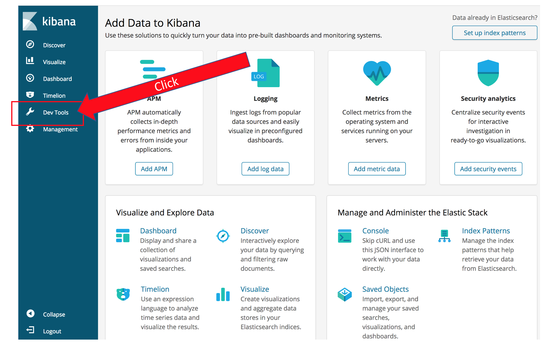
In Kibana’s main screen, select the Dev Tools tab
Click Get to work
The panel you now see lets you send requests directly to Amazon Elasticsearch Service. You enter the HTTP method, and the URL body. Kibana starts out with a helpful example. Click the  to execute the query and you should see Elasticsearch’s response in the right half of the screen.
For your first query, you will search the movie titles for Iron Man. Click after the closing bracket for the _matchall query and hit Enter a couple of times to get some blank lines.
Type “GET”. Notice that Kibana provides a drop down with possible completions. Finish typing out (or copy-paste) the following query
GET movies/_search
{
 "query": {
 "match": {
 "title": "star wars"
 }
 },
 "_source": "title"
}
Let’s dissect the results:
{
 "took": 23,
 "timed_out": false,
 "_shards": {
 "total": 1,
 "successful": 1,
 "skipped": 0,
 "failed": 0
 },
 "hits": {…
The top section contains metadata about the response. Elasticsearch tells you that it took 23 ms (server side) to complete the query. The query didn’t time out. Finally it gives you a report on the engagement of the shards: 1 total shard responded, successfully.
The hits section contains the actual search results. In the query, you specified _source: “title” in your query, so Elasticsearch returns only the title for each of the hits. You can specify an array of fields you want retrieved for _source or leave it off to see the full, source records.
Search multiple fields
One of Elasticsearch’s strengths is that it creates an index for the values of every field. You can use those indexes to construct complex queries across all of your data.
The bool query allows you to specify multiple clauses along with logic for combining results that match those clauses. You specify fields and values that must match in the must section. All must clauses must match for a document to match the query. These clauses represent a Boolean AND. You can also specify fields and values that should match – representing a Boolean OR. Finally you can specify fields and values that _mustnot match (Boolean NAND).
Enter the following query in the left pane of Kibana’s Dev Tools pane:
GET movies/_search
{
    "query": {
        "bool": {
            "must": [
                {
                    "term": {
                        "actors.keyword": {
                            "value": "Mark Hamill"
                        }
                    }
                },
                {
                    "range": {
                        "running_time_secs": {
                            "gte": "6000"
                        }
                    }
                },
                {
                    "range": {
                        "release_date": {
                            "gte": "1970-01-01",
                            "lte": "1980-01-01"
                        }
                    }
                }
            ],
            "should": [
                {
                    "range": {
                        "rating": {
                            "gte": 8.0
                        }
                    }
                }
            ]
        }
    }
}
Spend some time experimenting with different fields and values. You can use Kibana’s auto-complete feature to help you figure out different query types (the above query uses term and range, but there are many more, including match, _matchphrase, and span.
Search based on geographic location
With Elasticsearch, you can use the numeric properties of your data natively. You’ve seen an example of this above, where we searched for a range of dates and ratings. Elasticsearch also handles location in several formats, including geo points, geo polygons, and geo hashes. The sample movie data includes locations, drawn from 100 American cities, and assigned at random. You can run a bounding-box query by executing the following:
GET movies/_search
{
    "query": {
        "bool": {
            "filter": {
                "geo_bounding_box": {
                    "location": {
                        "top_left": {
                            "lat": 50.96,
                            "lon": -124.6
                        },
                        "bottom_right": {
                            "lat": 46.96,
                            "lon": -120.0
                        }
                    }
                }
            }
        }
    },
    "sort": [
        {
            "_geo_distance": {
                "location": {
                    "lat": 47.59,
                    "lon": -122.43
                },
                "order": "asc",
                "unit": "km"
            }
        }
    ]
}
This query searches a bounding box around Seattle and sorts the results by their distance from the center of Seattle. Even though the results themselves are not particularly meaningful (the locations are randomly assigned), the same method will let you search and sort your own data to display results that are geographically local for your customers.
Search free text
Elasticsearch’s features make it easy for you to search natural language text in a language-aware way. It parses natural language text, applies stemming, stop words, and synonyms to make text matches better. And has a built-in notion of scoring and sorting that brings the best results to the top.
The sample data includes a plot field with short descriptions of the movies. This field is processed as natural language text. You can search it by entering the following query:
GET movies/_search
{
    "query": {
        "match": {
            "title": "star man"
        }
    },
    "_source": "title"
}
You’ll see that you get a mix of movies, including Star Wars, Star Trek, and a couple of others. By default the match query uses a union (OR) of the terms from the query, so only one term is required to match. You could change the query to be a bool query and force both star and man to match. Let’s instead experiment with the scoring.
GET movies/_search
{
    "query": {
        "function_score": {
            "query": {
                "match": {
                    "title": "star man"
                }
            },
            "functions": [
                {
                    "exp": {
                        "year": {
                            "origin": "1977",
                            "scale": "1d",
                            "decay": 0.5
                        }
                    }
                },
                {
                    "script_score": {
                        "script": "_score * doc['rating'].value / 100"
                    }
                }
            ],
            "score_mode": "replace"
        }
    }
}
You’ve added an exponential decay function, centered on the year 1977. You’ve also used a script to multiply Elasticsearch’s base score by a factor of each document’s rating. This brings Star Wars to the top and sorts the rest of the movies mostly by their release date.
Retrieve aggregations
Elasticsearch’s aggregations allow you to summarize the values in the fields for the documents that match the query. When you’re providing a search user interface, you use aggregations to provide values that your users can use to narrow their result sets. Elasticsearch can aggregate text fields or numeric fields. For numeric fields, you can apply functions like sum, average, min, and max. The ability to aggregate at multiple levels of nesting is the basis of Elasticsearch’s analytics capabilities, which we’ll explore in the next section. Try the following query:
GET movies/_search
{
    "query": {
        "match_all": {}
    },
    "aggs": {
        "actor_count": {
            "terms": {
                "field": "actors.keyword",
                "size": 10
            },
            "aggs": {
                "average_rating": {
                    "avg": {
                        "field": "rating"
                    }
                }
            }
        }
    },
    "size": 0
}
Your results will show you a set of buckets (aggs) for actors, along with a count of the movies they appear in. For each of these buckets, you will see a sub-bucket that averages the ratings field of these movies. This query also omits the hits by setting the size parameter to 0 to make it easier to see the aggregation results.
You can experiment with building aggregations of different types and with different sub-buckets.
Stream updates to DynamoDB
In your web browser, open a new tab for https://console.aws.amazon.com and choose Lambda
Select Functions in the left pane
You will see the three Lambda functions that the lab deploys, named <stack name>-WiringFunction-<string>, <stack name>-LambdaFunctionForDDBStreams-<string>, and <stack name>-StreamingFunction-<string>. Click <stack name>-StreamingFunction-<string>
This function will generate random updates for the clicks and purchases fields, and send those updates to DynamoDB. These updates will in turn be shipped to Amazon ES through the LambdaFunctionForDDBStreams. If you examine the code, you’ll see that the function ignores its input and simply runs in a loop, exiting just before it times out
Click Test
Type an Event Name
Since the inputs don’t matter, you don’t have to change them. Click Create
Click Test. This will run for 5 minutes, streaming changes to Amazon ES via DynamoDB
Analyze the changes with Kibana
If you examine the code for the LambdaFunctionForDDBStreams, you’ll see that when data is modified in your DynamoDB table, the function sends both the update and a log of the changes to the clicks and purchases to a logs-<date\> index. You can use Kibana to visualize this information.
Return to your Kibana tab (or open a new one)
Click Management in the navigation pane
Click Index Patterns. You use index patterns to tell Kibana which indexes hold time-series data that you want to use for visualizations
In the Index Pattern text box, type logs (leave the ***** that Kibana adds automatically)
Kibana reports Success in identifying an index that matches that pattern
Click Next Step
Here you tell Kibana which field contains the time stamp for your records. Select @timestamp from the Time filter field name drop down
Click Create Index Pattern
Kibana recognizes the fields in your index and displays them for you
Click Discover in the navigation pane
This screen lets you view a traffic graph (the count of all events over time) as well as search your log lines for particular values

(Note, you can see my data covers 5 minutes and then stops. That’s because the Lambda function that’s streaming changes terminates. You can go back to the Lambda console and click Test again to stream more changes)
You can also use Kibana to build visualizations and gather them into a dashboard for monitoring events in near real time
Click Visualize in the navigation pane
Click Create a visualization You can see that Kibana has many different kinds of visualizations you can build
Click Line
On this screen, you tell Kibana which index pattern to use as the source for your visualization. Click logs*
When building Kibana visualizations you will commonly put time on the X-axis and a function of a numeric field on the Y-axis to graph a value over time
In the Buckets section, click X-Axis
In the Aggregation drop down, select Date Histogram
Click  to change the visualization. You now have a graph of time buckets on the X-Axis and the Count of events on the Y-Axis
In the Aggregation drop down for the Y-Axis, select Sum and in the Field drop down, select purchases to see the sum of all purchases, broken down by time
You can monitor changes in this metric, in near real time, by clicking  in Kibana’s top menu bar, and choosing 10 seconds. Kibana now updates every 10 seconds. You might have to start the Lambda stream function again to generate more data or you might see data continuing to flow in
You can save your visualizations and build them into dashboards to monitor your infrastructure in near real time.
Clean up
When you’re done experimenting, return to the CloudFormation dashboard
Click the check box next to your stack, then choose Delete Stack from the Actions menu
Click Yes, Delete in the dialog box.
Conclusion
In this lab, you used CloudFormation to deploy a DynamoDB table, and an Amazon Elasticsearch Service domain to search the data in your table. You explored building complex, bool queries that used the indexes for your fields’ data. You explored Elasticsearch’s geo capabilities, and its abilities to search natural language data. You created aggregations to analyze the movie data and discover the best-rated actor in this data set. Finally, you used DynamoDB streams to flow updates from your table to your domain and Kibana to visualize the changes in your table.
Whew! That’s a lot! And you’ve barely scratched the surface of Elasticsearch’s capabilities. Feel free to use this lab guide and its template to explore more on your own.